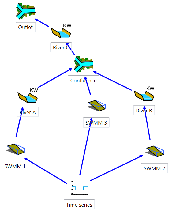
In the first example the objective is to model the production of a net rain-flow of three impermeable basins, then the propagation of two hydrographs, the implementing of three inflows at a confluence and finally their propagation to the model outlet (Figure 16.1).

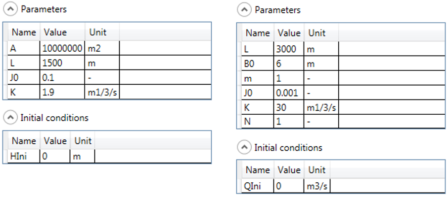
The three impermeable surfaces are supposed to be located in the same region, thus receiving an identical precipitation. Each surface has its own outlet into different rivers (A and B) which are joined later on in a single final river (C) before flowing into the outlet of the model. The parameters and the state variables of the three surfaces, of the three rivers and the precipitation data are provided in Figure 16.2. The three rivers are modeled with the kinematic wave model.
16.1 Objective of Example 1
The requested result is the hydrograph at the model outlet during 24 hours, after the beginning of the precipitation, as well as the peak discharge and the peak time.
The simulation parameters are:
Simulation time step = 600 s
Recording time step = 600 s
A uniform and null ETP is assumed for this example (the user can check the selected ETP method in the RS MINERVE settings).

16.2 Resolution of Example 1
This first example is a simplified representation of the reality. Despite of that, it allows the familiarization with the concept of RS MINERVE and to know more about its hydrological objects.
At first, the object “Time Series” ![]() is introduced. Clicking once on its icon in the Objects frame, a pen appears. You can then click in the graphic interface for creating the object in the position you want. Next, the three run-off surfaces are created by means of the object “SWMM”
is introduced. Clicking once on its icon in the Objects frame, a pen appears. You can then click in the graphic interface for creating the object in the position you want. Next, the three run-off surfaces are created by means of the object “SWMM” ![]() . The three rivers are introduced by selecting the model “Kinematic Wave”
. The three rivers are introduced by selecting the model “Kinematic Wave” ![]() . The model built-up will be finished with the introduction of the two objects “Junction”
. The model built-up will be finished with the introduction of the two objects “Junction” ![]() .
.
The graphical interface at this stage is presented in Figure 16.3.

After creating the new objects, topological links or connections have to be established. To do so, it is sufficient to press once the space bar of the keyboard to pass in “connections” mode. In Editing tools, the Connections button is then automatically pressed (Figure 16.4). Flying over each objet, the curser presented before as an arrow now appears as a cross. Next, click from the object “Time Series” to the object “SWMM1”, thus creating a topological link.

The others objects are connected in the same way. Press again the space bar of the keyboard to return to selection mode. The construction of all the model objects and the resulting topologic links is thus achieved as presented in Figure 16.5 and it only remains the introduction of the parameters.
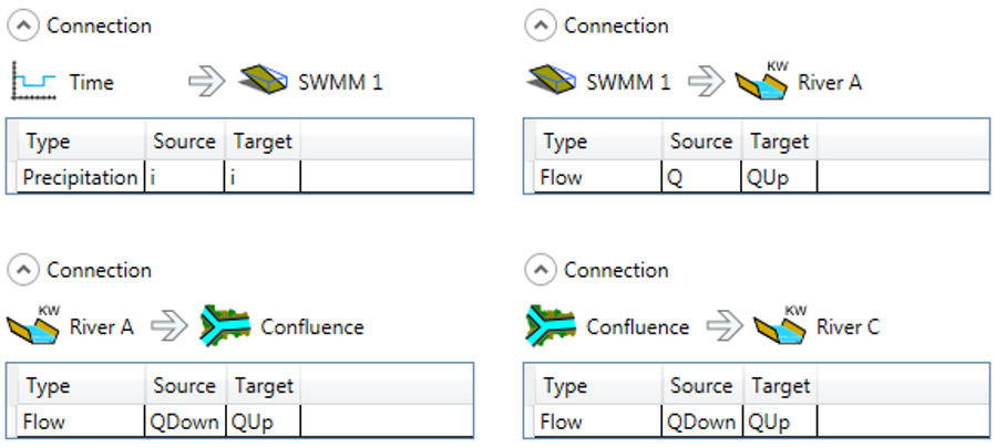
By double clicking on the links just created (blue arrows), the information transferred between “Time Series” and the three run-off surfaces as well as that between all other objects from up- to downstream is verified (Figure 16.6).
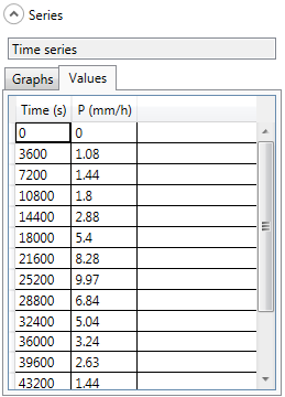
In clicking double on the Time Series object, the associated frame is opened on the right of the screen and the values “Time (s) - P (mm/h)” are introduced (Figure 16.7).
Next, for each SWMM object (![]() ), the respective parameters (values available in Figure 16.2) are defined by double clicking on every object and introducing them by the help of the both Parameters and Initial conditions frames. The parameters of the Rivers are introduced in the same way (Figure 16.8).
), the respective parameters (values available in Figure 16.2) are defined by double clicking on every object and introducing them by the help of the both Parameters and Initial conditions frames. The parameters of the Rivers are introduced in the same way (Figure 16.8).
The date parameters of the simulation are modified in Solver frame on the left of the screen (Figure 16.9) before the calculation. For both dates “Start” and “End” an arbitrary date is proposed, but the “End” date has to finish 24 hours later than “Start” date. The “Simulation time step” and the “Recording time step” have a value of 600 s.

Constructed final model can be now saved clicking in the button ![]() and giving a name to the file (e.g. “Example1.rsm”). This way the model could be loaded later to do new simulations (Figure 16.10).
and giving a name to the file (e.g. “Example1.rsm”). This way the model could be loaded later to do new simulations (Figure 16.10).

Before running calculation, a pre-simulation validation of the model parameterization can be made in clicking in the button ![]() (Solver frame). Its report is summarized on the right of the interface.
(Solver frame). Its report is summarized on the right of the interface.
Finally, the simulation is initiated by clicking on the button Start in the Solver frame.
16.3 Results of Example 1
In order to access to the calculation results for each object it has to be clicked two times on any of them. For example, clicking double on the object Outlet, its dialog box is opened on the right and the simulated hydrograph, being the objective of the Example 1, is shown (Figure 16.11).
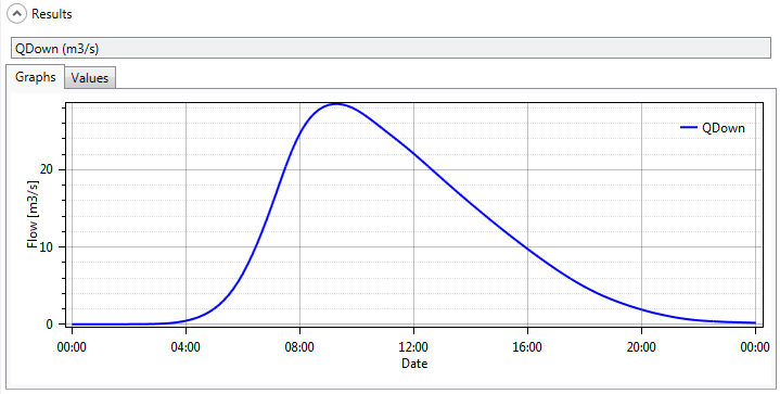
If we check the values (Figure 16.12), we can found that the maximal discharge (28.442 m3/s) arrives at 09:20 (assuming the simulation starts at 00:00).
